AutoGRAPH - Tutorial |

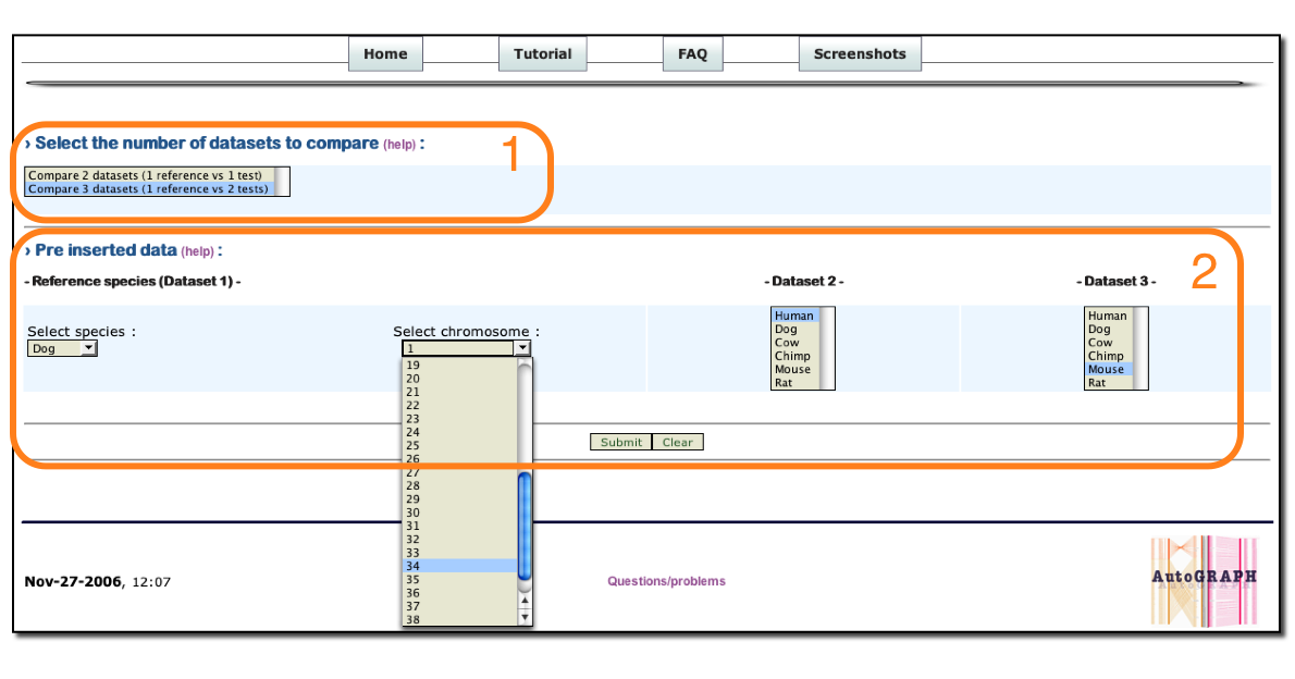
1 : Select the number of species to compare.
2 : Select one Reference species and the reference chromosome (or all chromosomes) and select species 2 and 3 to be compared.
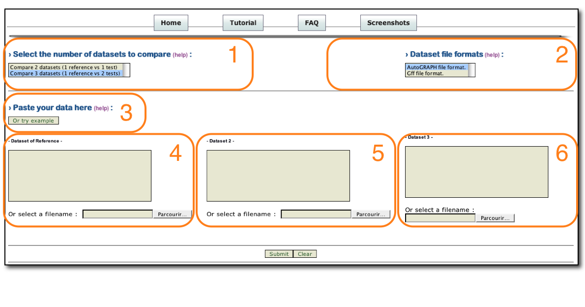
1 : Select the number of species to compare.
2 : Select input file formats. (* see below for description)
3 : Click to get an example of text input format to launch AutoGRAPH.
4 : Paste reference dataset or browse your file ( or see example in order to integrate 2 resources within one species -here- ).
5 : Paste dataset 2 or browse your file.
6 : Paste dataset 3 or browse your file.
i. AutoGRAPH file format: rows must be formatted as:
- <marker_identifier> <chromosome> <position> - (example)
Each column should be separated by space(s) or tab.
ii. GFF file format: rows must be formatted as:
- <seqname> <source> <feature> <start_position> <end_position> <score> <strand> <frame> - (See description of gff format on Sanger web site)
AutoGRAPH parses input gff files and stores useful data (i.e seqname, source, feature, start and strand) in order to build comparative map.
Concerning the gff semantic, we define "feature" item as the chromosome Id.
Missing data should be set by a dot '.'. Each column should be separated by space(s) or tab.
One raw Example : "ENSCAFG00000014677 ENSEMBL_GeneWise CFA_34 37451049 37453338 . - 1".
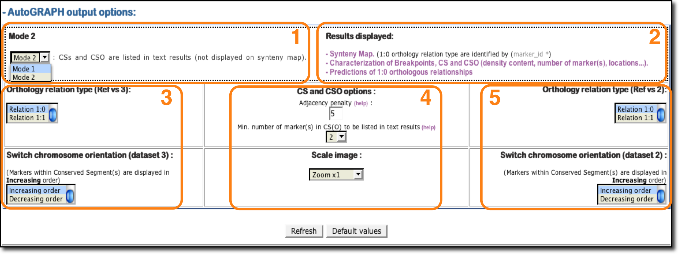
1: Mode (1/2): Mode option allows user to set the comparative map to be displayed. Mode 1 permits to define 1:1 orthologous relationships and Mode 2 allows 1:1 and 1:0 orthologous anchors to be analyzed.
2: Results displayed: Click on each links to get results. Three possibilities are available: Synteny map (mode 1/2), characterization of breakpoints, CS and CSO (mode 1/2) and predictions of 1:0 relationships (mode 2).
3: Dataset 3 options : Options allows user to modify the orthology relationships displayed on synteny map (mode 1 -› 1:1 and mode 2 -› 1:1/1:0) and to change the orientation (increasing/decreasing) of the dataset 3 in the figure.
4: CS and CSO options:
- Adjacency penalty: It correponds to a number of genes/markers set by users that permits to identify an interruption in the colinearity of a Conserved Segment (more info).
- Minimum number of markers listed in array results: Select the minimum number of markers/anchors to define a CS(O) and to be listed.
These informations are stored and displayed in the results array at the bottom of the figure and in a flat-file that can be downloaded.
5: Dataset 2 options : Options allows user to modify the orthology relationships displayed on synteny map (mode 1 -› 1:1 and mode 2 -› 1:1/1:0) and to change the orientation (increasing/decreasing) of the dataset 2 in the figure.
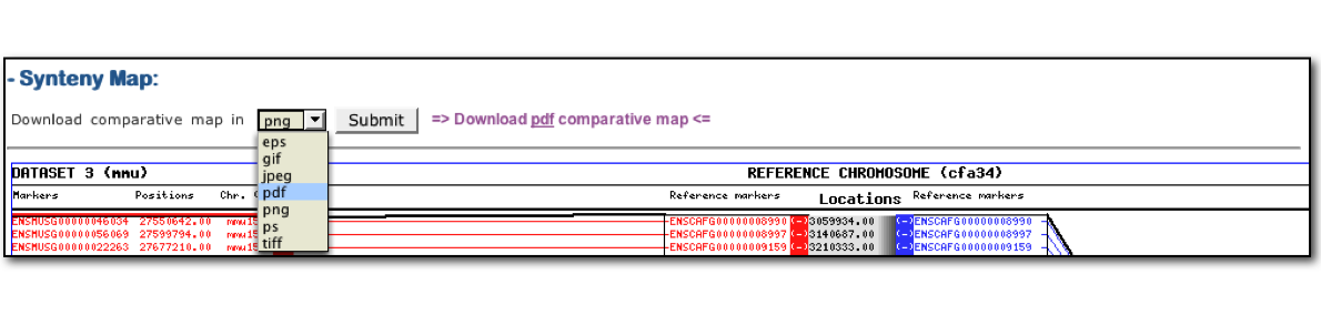
User can save their output comparative map in several formats included .png, .gif, .jpeg as well as .pdf, ps, .eps...
- Download the output_tutorial to interprete an example output corresponding to the comparison of canine chromosome 34 (CFA 34) with human and mouse genomes.
- Or click on images to see how interpreting results for the same example: